
Tamas Koncz


Welcome to the first post in my ‘The Big Bang Theory (Tidy)Text analysis’ mini-series, and with that, to the very first post on my blog!
Recently I was taking a class on ‘Data Science on Unstructured Text Data’, for which our final project was to create a tidyverse text analysis of any topic of our choice.
While originally I set my sight on some deep topics, I ended up with something lighter this time. What you need to know about me is that I’m quite addicted to spending my time in front of different TV series. TBBT used to be one of my favorites - and while the series lost some of its brilliance over the years, I still thought its body of many seasons should be great material for my analysis (also, lucky for me, Silicon Valley can fill in for my need of some good nerdy humor).
For this post what I was interested in is if the frequency of certain names appearing has some connection to an episode’s success (in this case, measured by the average rating of users on IMDB).
For the purposes of this excercise, names can appear in any format - the point is characters being mentioned in one way or another.
During this post, I’ll share bits of code to guide through my analysis - if you are interested in more, please refer to my github page.
Let’s dive into the details!
The data originally looked like as below1. The full spoken text for each episode was one row, marked by ‘episode_id’. The data did not contain any metadata about speakers, or any contextual information, just the senteces that characters said during the show.
A glimpse into how it looked when I started:
| episode_id | episode_full_text |
|---|---|
| s1e1 | So if a photon is directed through a plane with two slits in it and either slit is observed, it will not go through both slit… |
| s1e2 | Here we go. Pad thai, no peanuts. But does it have peanut oil? I’m not sure. Everyone keep an eye on Howard in case he starts… |
| s1e3 | Alright, just a few more feet. And… here we are, gentlemen, the Gates of Elzebob. Good Lord. Don’t panic. This is what the … |
The first step I had to do is extract all words from the above format, using the unnest_tokens function:
words_by_episode <- full_episode_text %>%
unnest_tokens(output = word, input = episode_full_text)| episode_id | word |
|---|---|
| s1e1 | so |
| s1e1 | if |
| s1e1 | a |
| s1e1 | photon |
| s1e1 | is |
The only “words” that I needed were the character names mentioned. However, simply selecting lines based on whether they contain names or not would not work.
Let’s consider the below examples of “sheldon” and “raj”:
words_by_episode %>%
  filter(str_detect(word, "raj")) %>%
  select(word) %>%
  unique() %>%
  rename("Lines containing 'raj'" = "word") %>%
kable()| Lines containing ‘raj’ |
|---|
| raj |
| rajesh |
| raj’s |
| trajectory |
| rajasthan |
| maharaja |
| rajesh’s |
| raj’ll |
words_by_episode %>%
  filter(str_detect(word, "sheldon")) %>%
  select(word) %>%
  unique() %>%
  rename("Lines containing 'sheldon'" = "word") %>%
kable()| Lines containing ‘sheldon’ |
|---|
| sheldon |
| sheldon’s |
| sheldonmano |
| sheldons |
| sheldonectomy |
| sheldonopolis |
| sheldonian |
| sheldonoscopy |
| sheldony |
We can see that names appear in many different format throught the text.
To handle this, I create a vector containing regular expressions, custom-made for each name. (For most names this is still simply the name - I had to review one-by-one to decide on the right approach.)
first_names_for_regex <- c("howard",     "penny",      "leonard",     "sheldon",
                           "^raj[e']?",  "^(sh)?amy",  "^bern[ias]",  "stuart",
                           "zack",       "emil[ey]",   "leslie",      "barry",
                           "priya",      "stephanie",  "lucy")
This vector can be merged into one regex, that we can use for filtering on the “word” column:
first_names_regex <- paste0(first_names_for_regex, collapse = '|')
first_names_regex <- paste("(", first_names_regex, ")", sep = "")

fnames_in_episodes <- words_by_episode %>%
                        filter(str_detect(word, first_names_regex))
Given formatting was all over the place (see below…), as a next step I’ve applied some standardization.
##  [1] "leonard"          "sheldon"          "penny"
##  [4] "sheldon's"        "howard"           "penny's"
##  [7] "raj"              "rajesh"           "leslie"
## [10] "leonard's"        "howard's"         "raj's"
## [13] "sheldonmano"      "barry"            "sheldons"
## [16] "stephanie"        "stephanie's"      "sheldonectomy"
## [19] "bernie"           "rajasthan"        "stuart"
## [22] "stuart's"         "leslie's"         "emile"
## [25] "bernadette"       "bernadette.she's" "bernadette's"
## [28] "sheldonopolis"    "zack"             "amy"
## [31] "amy's"            "shamy"            "sheldonian"
## [34] "priya"            "priya's"          "zack's"
## [37] "bernie's"         "rajesh's"         "leonardville"
## [40] "leonardstan"      "leonardwood"      "leonards"
## [43] "koothrapenny"     "emily"            "raj'll"
## [46] "amygdala"         "lucy"             "lucy's"
## [49] "emily's"          "sheldonoscopy"    "koothrapemily"
## [52] "amyâ"             "sheldony"         "pennysaver"
## [55] "amy.â"            "bernstein"        "howardâ"
## [58] "leonardo"         "emily.â"          "emilyâ"
## [61] "bernardino"       "bernatrix"
first_names <- c("Howard", "Penny", "Leonard", "Sheldon",
"Raj", "Amy", "Bernadette", "Stuart",
"Zack", "Emily", "Leslie", "Barry",
"Priya", "Stephanie", "Lucy")
first_names_mapping <- data.table(regex = first_names_for_regex,
name = first_names)
len_first_names_mapping <- first_names_mapping %>% nrow()
fnames_in_episodes$name <- ""
for(i in c(1:len_first_names_mapping)) {
fnames_in_episodes <- fnames_in_episodes %>%
mutate(name = ifelse(str_detect(word, first_names_mapping[i, regex]),
first_names_mapping[i, name],
name))
}A small glimpse into the format we arrived at:
fnames_in_episodes %>%
  filter(name == "Leonard") %>%
  select(word, name) %>%
  unique() %>%
kable()| word | name |
|---|---|
| leonard | Leonard |
| leonard’s | Leonard |
| leonardville | Leonard |
| leonardstan | Leonard |
| leonardwood | Leonard |
| leonards | Leonard |
| leonardo | Leonard |
Let’s count how many times names appear per episode, and then spread the dataset to the wide format, which can be fed into a predictive model:
episodes <- fnames_in_episodes %>%
              select(-word) %>%
              group_by(episode_id, name) %>%
              summarize(name_appear_count = n()) %>%
              tidyr::spread(key = name, value = name_appear_count, fill = 0)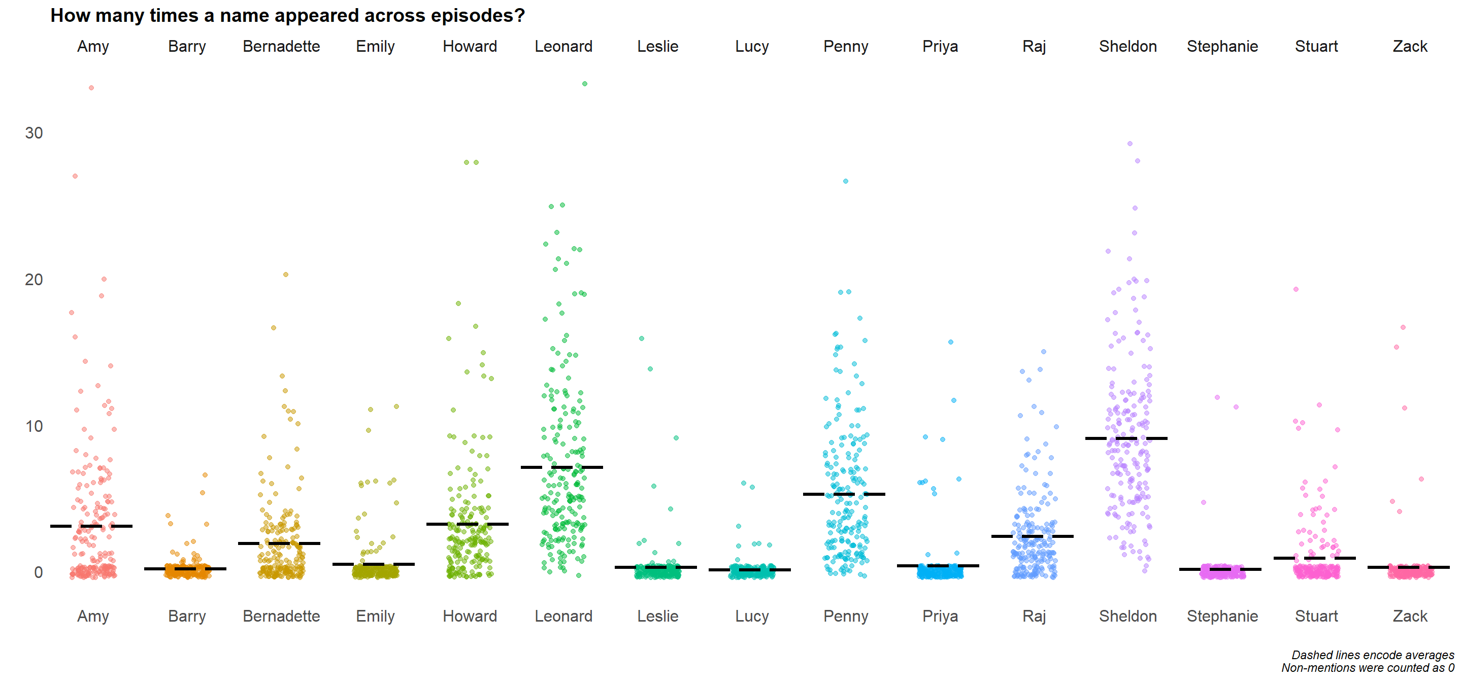
We can then just join the IMDB scores based on episode ids:2
episodes_w_scores <- imdb_scores %>%
                       inner_join(episodes, by = "episode_id") %>%
                       select(-Season, -Episode, -Title)
Now that the data is in shape, it’s time to do what we are here for - figuring out who has the best impact on those IMDB scores!
My approach here is very simple: I’m going to run a glm regression, with on a training set of 75% of the original data. The remaining 25% will be used as a validation set, that helps ensure that the model did not overfit.
The goal is not to build the best predictive model, as what I’m interested in is the coefficients. The simpler model, the more interpretable they will be.
training_ratio <- 0.75

set.seed(93)
train_indices <- createDataPartition(y = episodes_w_scores[["IMDB Score"]],
                                     times = 1,
                                     p = training_ratio,
                                     list = FALSE)

data_train <- episodes_w_scores[train_indices, ]
data_test  <- episodes_w_scores[-train_indices, ]
train_control <- trainControl(method = "none")
set.seed(93)
glm_fit <- train(`IMDB Score` ~ . -episode_id,
method = "glm",
data = data_train,
trControl = train_control,
preProcess = c("center", "scale"))When I ran the model I deemed it good enough to draw some conclusions, so it’s time to take a look at those coefficients (see end notes on model robustness).
coefficients <- coef(glm_fit$finalModel)[-1]
coefficients <- data.frame(Name      = names(coefficients),
                           beta      = coefficients,
                           row.names = NULL) %>%
                mutate(Name = reorder(Name, beta)) %>%
                mutate(Impact = ifelse(beta >= 0, "+", "-"))
Putting the results into a nice visual:
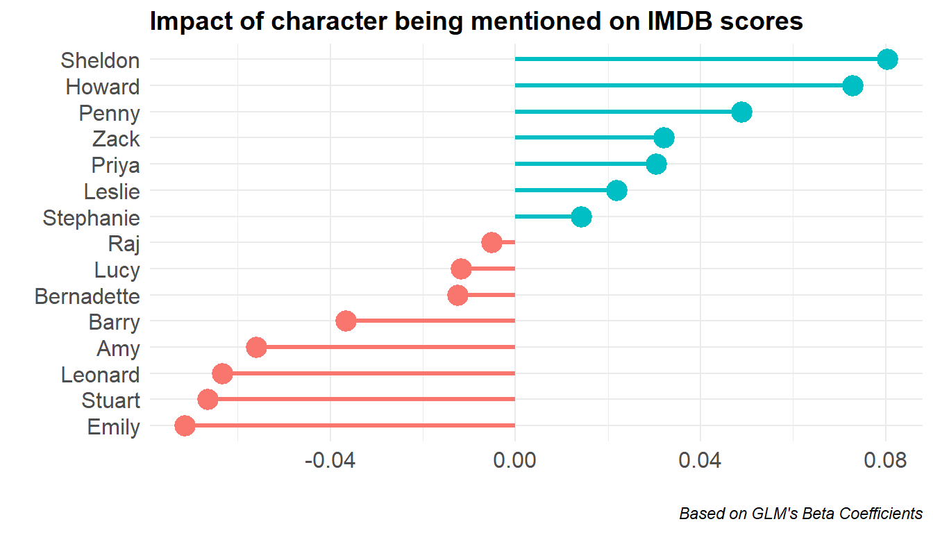
Let’s interpret the above: the most positive impact comes from Sheldon, Howard, and Penny, while the most negative is from Emily, Stuart, Leonard, and Amy.
Every time Sheldon is mentioned in some context, we expect an 0.08 higher IMDB score for the given episode. Every time Amy is mentioned in some context, we expect an 0.06 lower IMDB score for the given episode. 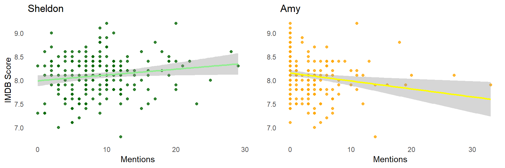
This should give us some insight into who are the viewer favorites of the show - but we should not take the results (just as the topic) too seriously.
The methodology is clearly not very robust - this is, after all, is more for fun than for “science”.
Notes:
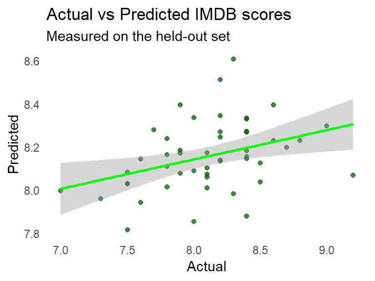
In the post I have not gone into detail about robustness of the model’s fit, so let’s spend a minute on that here.
One thing to look at is the RMSE on the set-aside test set vs the standard deviation of IMDB Scores:
## [1] "RMSE: 0.4, Std. Dev.: 0.43"That the values are in the same ballpark signals that even if just weakly, but the model does have some descriptive power.
I’m working on a post that describes how to gather subtitle data and turn it into a tidy format.↩
Data was downloaded from https://www.opensubtitles.org/en/ssearch/sublanguageid-eng/idmovie-27926, where they nicely collected live IMDB scores for all episodes of TBBT.↩